4.5.8 Coverage

Purpose

Analyze how Ribo-seq or RNA-seq density is distributed across normalized 5' UTR, CDS, and 3' UTR regions. Coverage analysis helps evaluate library quality, nuclease bias, mapping artifacts, and whether gene-level quantification can be trusted.

rpf_Coverage     # Normalize transcripts into bins and draw metagene coverage line plots, heatmaps, and barplots
rpf_Percent      # Calculate transcript-level CDS coverage percentages and draw histograms/boxplots
merge_coverage   # Merge mean coverage tables from multiple samples or analyses

Both current JSONL density files and the legacy TXT density files are supported. The workflow normalizes 5' UTR, CDS, and 3' UTR into a user-defined number of bins (-b), aggregates the binned density per sample, and outputs coverage tables together with line plots, a combined sample heatmap, and optional covered-transcript percentage barplots.

Step 1: Run rpf_Coverage

Normalize transcripts into bins and generate metagene coverage profiles from a merged density file.

1.1 Parameters

Parameter	Required	Description
-r, --rpf	Yes	Input RPF density file in JSONL or TXT format, usually the merged density file generated by rpf_Merge.
-o, --output	Yes	Output prefix.
-t, --transcript	No	Optional transcript filter table in TXT format. When provided, transcript_id is used if available.
-f, --frame	No	Reading frame used for coverage calculation. Choices are 0, 1, 2, and all. Default is all.
--site	No	Ribosomal site used for codon-level density shifting. Choices are E, P, A, and all. Default is P.
-m, --min	No	Retain transcripts with at least this sample-specific CDS RPF count. Default is 50.
--set	No	Transcript-region filtering strategy. union treats missing region bins as zero; intersect keeps only transcripts with all requested regions. Default is union.
--thread	No	Reserved for compatibility; the current coverage aggregation is vectorized. Default is 1.
-b, --bin	No	Bin numbers for 5' UTR, CDS, and 3' UTR, formatted as utr5,cds,utr3. Default is 30,100,30.
-n, --normal	No	Normalize RPF counts to RPM before coverage aggregation. Disabled by default.
--mode	No	Coverage plot type. both draws line plots and the combined sample heatmap. Choices are line, heatmap, both, and all. Default is both.
--plot-transform	No	Transform plotted density values without changing output tables. Choices are none, sqrt, log, log1p, log2, log10. log is an alias of log1p. Default is none.
--scale	No	Heatmap scaling method. row applies row-wise min-max scaling to emphasize each sample profile shape. Choices are none and row. Default is none.
--bar	No	Draw covered-transcript percentage barplots. Disabled by default.
--remove-outlier, --outlier	No	Remove extreme transcript-bin RPF pileups before aggregation. Useful for rRNA-like or mis-mapped fragments. Disabled by default.
--outlier-iqr	No	IQR multiplier for extreme pileup detection. Default is 8.0.
--outlier-window	No	Number of neighboring bins on each side used to estimate local background. Default is 5.
--outlier-local-fold	No	Minimum fold over local background for dynamic isolated-pileup filtering. Default is 10.0.
--gene-heatmap, --heat	No	Deprecated compatibility option and will be ignored. The combined sample heatmap is controlled by --mode heatmap/both/all.

1.2 Example

cd ./sce/4.ribo-seq/08.coverage/

rpf_Coverage \
    -t /path/to/norm/sce.genepred \
    -r ../05.merge/sce_rpf_merged.jsonl.gz \
    -m 50 \
    --outlier \
    -b 10,100,10 \
    -n \
    --bar \
    --plot-transform sqrt \
    -o sce \
    &> sce.log

1.3 Output

Output	Description
<prefix>_metagene_coverage.txt	Binned metagene coverage table for all samples.
<prefix>_metagene_coverage_percentage.txt	Covered-transcript percentage table. Written when --bar is used.
<prefix>_coverage.sample_summary.txt	Per-sample summary of the coverage aggregation.
<prefix>_coverage.outliers.txt	Outlier table listing removed pileup points. Only written when --remove-outlier is enabled.
<prefix>_coverage.summary.json	Machine-readable summary of the run, including the output file list.
<prefix>_coverage_line_plot.pdf / .png	Combined average coverage line plot over all samples.
<prefix>_{sample}_coverage_line_plot.pdf / .png	Per-sample coverage line plot (one file per sample).
<prefix>_coverage_heatmap.pdf / .png	Heatmap of all sample coverage profiles, drawn when --mode heatmap/both/all.
<prefix>_{sample}_coverage_bar_plot.pdf / .png	Per-sample covered-transcript percentage barplot (one file per sample). Written when --bar is used.

Example output figures

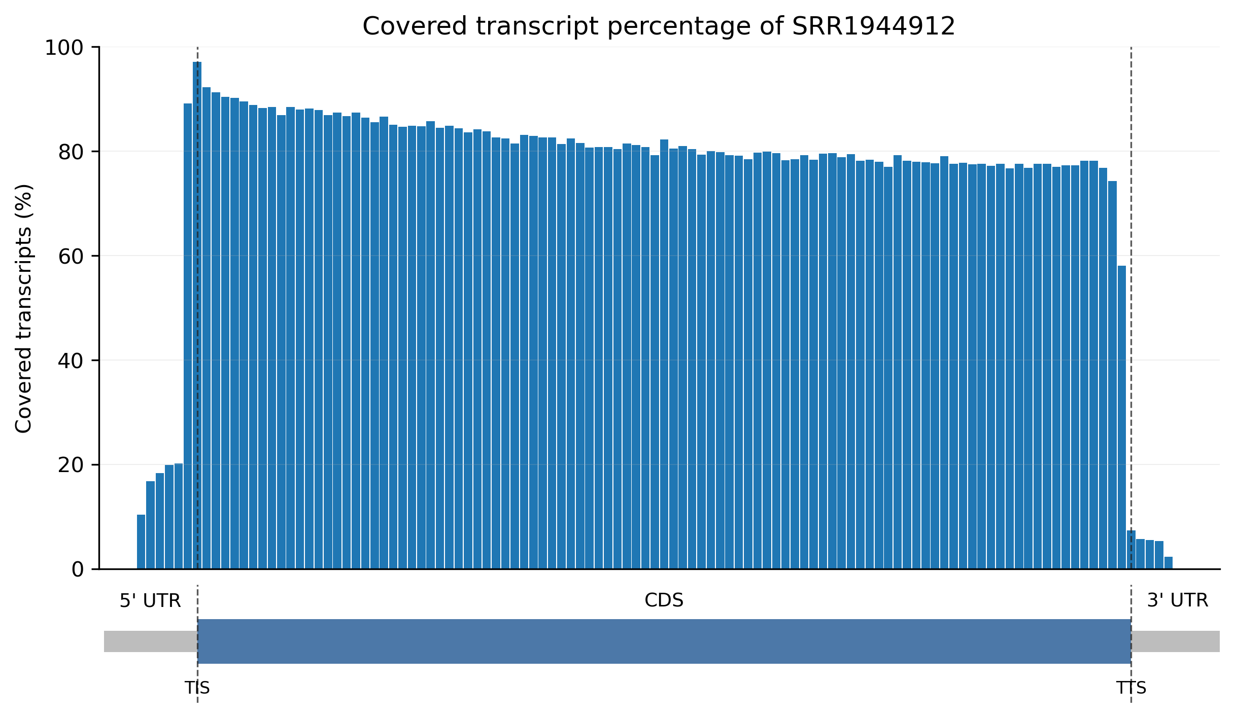
Coverage barplot for a single sample (sce_SRR1944912_coverage_bar_plot.png). The x-axis shows the normalized 5' UTR, CDS, and 3' UTR bins; the y-axis shows the average RPF density per bin. In a high-quality library, the CDS should show uniform coverage, while peaks at the translation initiation site (TIS) and translation termination site (TTS) are expected Ribo-seq signals caused by ribosome stalling:

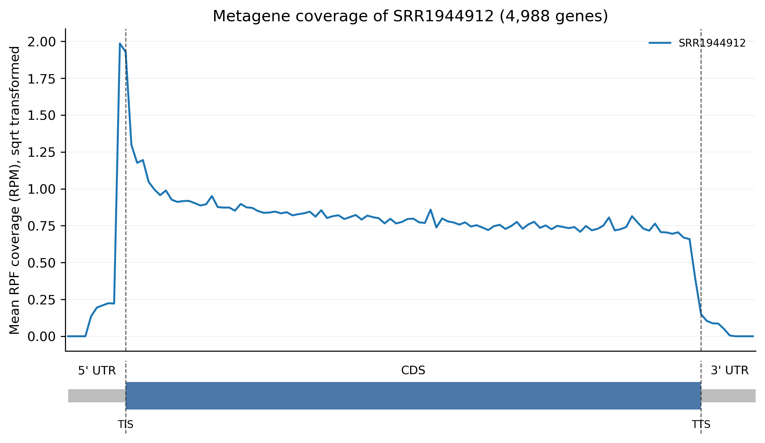
Coverage line plot for a single sample (sce_SRR1944912_coverage_line_plot.png). It provides the same information as the barplot but with a continuous line, which makes it easier to inspect the shape of the 5' UTR, CDS, and 3' UTR profiles and to compare subtle differences between regions:

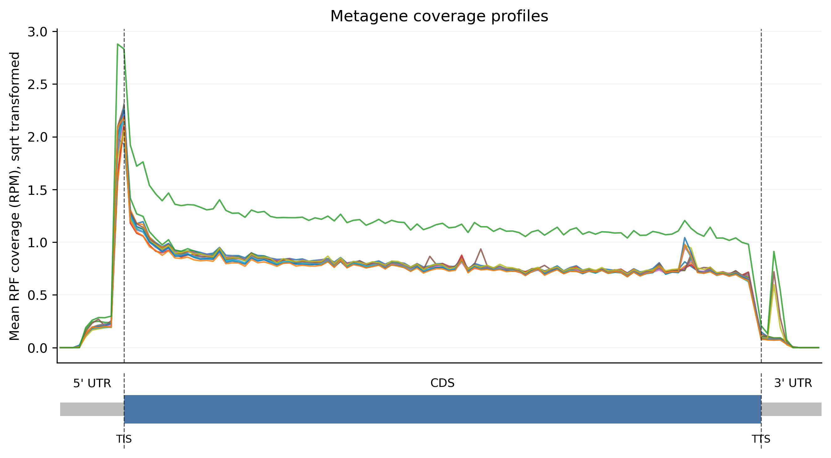
Combined coverage line plot for all samples (sce_coverage_line_plot.png). All sample profiles are overlaid in one figure, which allows a direct cross-sample comparison of the overall coverage shape. Consistent profiles suggest similar library quality, whereas one sample deviating from the others may indicate a library-specific bias:

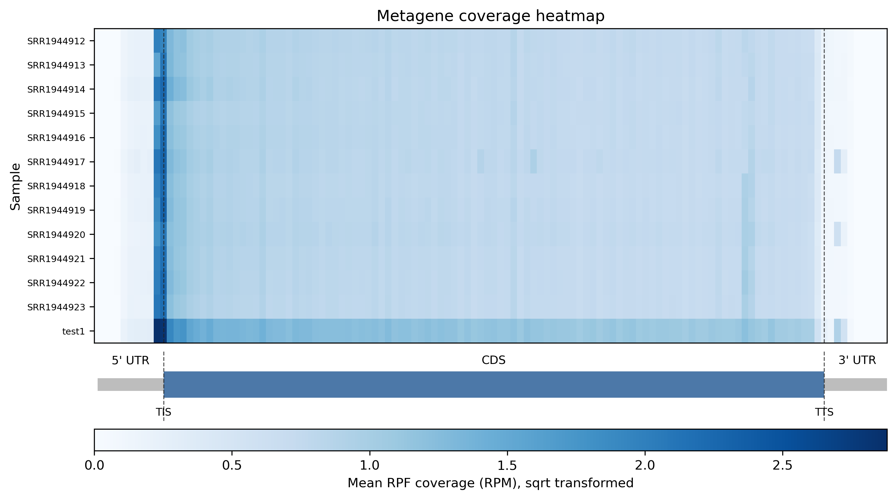
Heatmap of the coverage profiles for all samples (sce_coverage_heatmap.png). Each row is a sample and each column is a normalized region bin. Row-wise scaling (--scale row) highlights the shape of each profile; bright bands at the TIS/TTS and a uniform CDS block indicate good ribosome footprint enrichment:

Step 2: Run rpf_Percent

Calculate the percentage of valid CDS codons covered by RPFs for each transcript and sample.

2.1 Parameters

Parameter	Required	Description
-r, --rpf	Yes	Input RPF density file in JSONL, JSONL.GZ, TXT, or TSV format.
-o, --output	No	Output prefix. Default: input RPF filename without the density suffix.
-t, --transcript	No	Optional transcript annotation or ID list. The transcript_id column is used when present; otherwise the first column is used.
-f, --frame	No	Reading frame used for coverage calculation. Choices are 0, 1, 2, and all. Default is all.
-m, --min	No	Minimum sample-specific CDS RPF count required for a transcript. Default is 50.
--tis	No	Number of CDS codons removed after TIS. Default is 0.
--tts	No	Number of CDS codons removed before TTS. Default is 0.
-n, --normal	No	Use RPM instead of raw RPF count in abundance plots and summaries. Disabled by default.
--fig-format	No	Figure output format. Choices are png, pdf, and both. Default is png.
--dpi	No	PNG resolution. Default is 300.
--font-size	No	Base figure font size. Default is 11.0.

2.2 Example

rpf_Percent \
    -r ../05.merge/sce_rpf_merged.jsonl.gz \
    -m 50 \
    -f all \
    -o sce \
    &> sce.log

2.3 Output

Output	Description
<prefix>_gene_coverage_percent.txt	Transcript-level CDS coverage percentage table.
<prefix>_gene_coverage_summary.txt	Coverage summary table.
<prefix>_{sample}_coverage_histogram.png / .pdf	Per-sample coverage percentage histogram (one file per sample).
<prefix>_coverage_boxplot.png / .pdf	Coverage percentage boxplot for all samples.

Example output figures

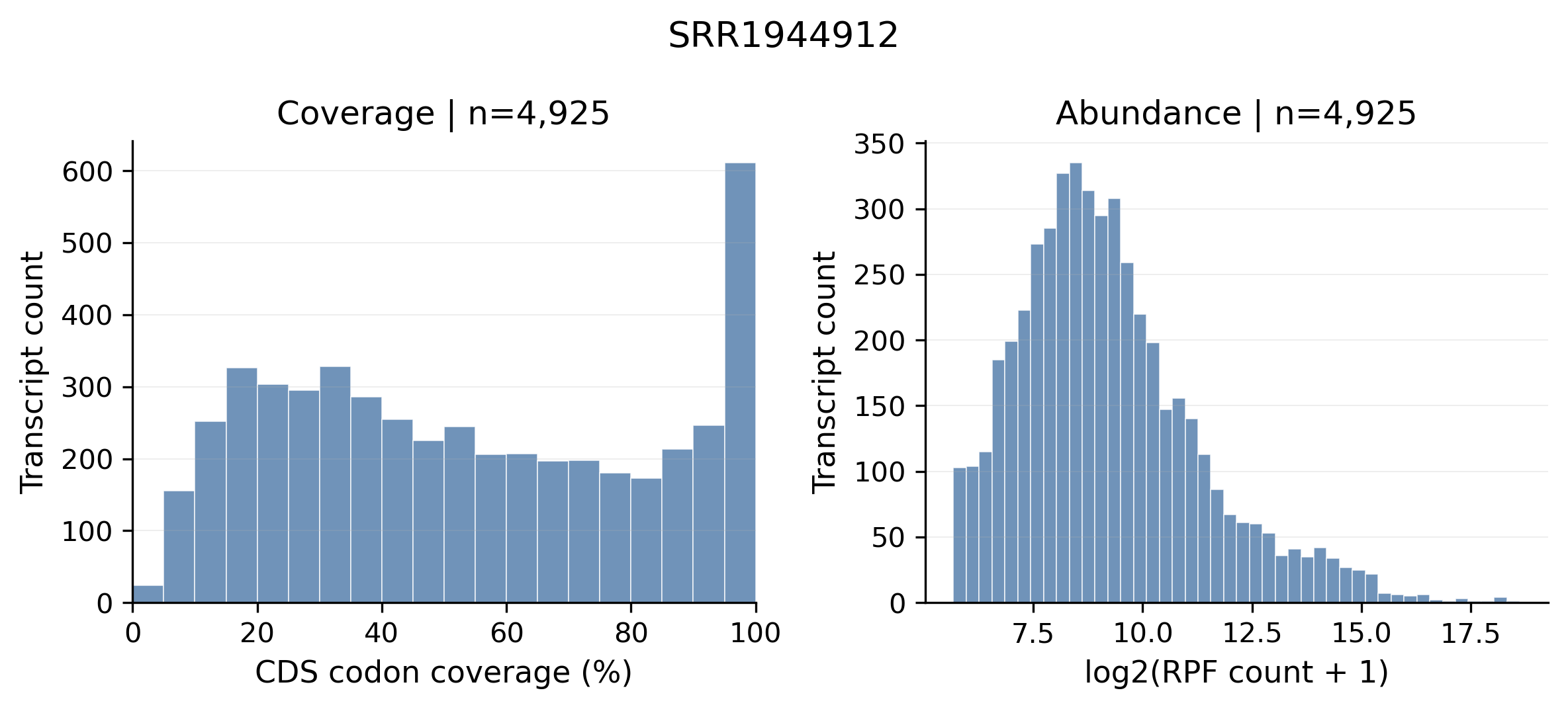
Coverage percentage histogram for a single sample (sce_SRR1944912_coverage_histogram.png). The x-axis is the percentage of valid CDS codons covered by RPFs per transcript, and the y-axis is the number of transcripts. A library with a strong right-skewed distribution (most transcripts clustered near high coverage percentages) indicates good CDS coverage and supports reliable gene-level quantification:

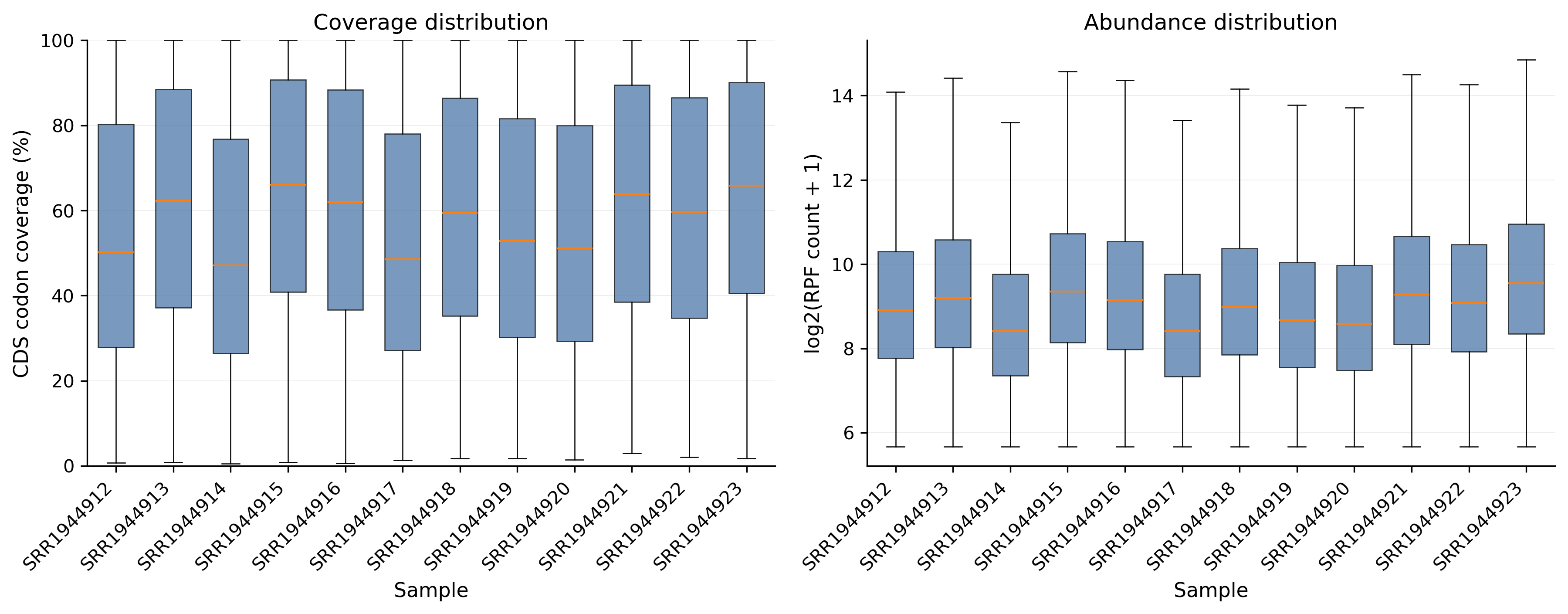
Coverage percentage boxplot for all samples (sce_coverage_boxplot.png). Each box summarizes the distribution of transcript-level coverage percentages in one sample. Samples with a higher median and a narrow box have more uniform coverage; large inter-sample differences suggest batch effects or library quality problems:

Step 3: Run merge_coverage

Merge mean coverage files from multiple samples or analyses into a single table.

3.1 Parameters

Parameter	Required	Description
-l, --list	Yes	Input coverage files, e.g. *_mean_coverage.txt. Multiple files can be provided.
-o, --output	Yes	Output prefix. The merged table is written to <prefix>_mean_coverage.txt.

3.2 Example

merge_coverage \
    -l *_mean_coverage.txt \
    -o sce

3.3 Output

Output	Description
<prefix>_mean_coverage.txt	Merged coverage table, concatenated from all input files, with columns Sample, Region, Bins, Density.

Notes

• Uniform CDS coverage supports reliable gene-level quantification, while strong 5' or 3' bias may reflect RNA degradation, nuclease bias, mapping artifacts, or library-specific structure.
• --plot-transform only changes how density values are displayed in figures; it does not alter the output tables.
• --gene-heatmap / --heat is deprecated and ignored. Use --mode heatmap or --mode both to draw the combined sample heatmap.
• Use consistent binning and filtering settings (-b, -m, --set) across samples when comparing coverage profiles.